Finding the Exponent in the Fiat Decay Model

In macroeconomics, the term “velocity of money” is often used. The concept is that money is reused as it passes from person to person so it must pass with some “velocity” (measured in exchanges per period).

A similar (but not identical) relationship is found in the model described in my post “Mapping Stimulus to GDP” . [In that post, the model had no name. In this post, the model will be label the Fiat Decay Model (FD Model).]  In the FD Model, the number of transactions is critical to establishing the limit of GDP expansion possible with any new fiat money supply. After each transaction, part of the new fiat issue is returned to government by taxation which leaves a diminished amount for further GDP expansion. Each transaction is treated as an increment of an exponent.

It is easy to find the velocity term in the common usage. Use the formula

Velocity = GDP/ Money Supply

where GDP is Gross Domestic Product.

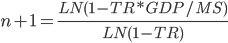
It is not so easy to find the exponent from the formula

(1)    - TR*GDP = - MS + MS*(1-TR)^(n+1)

(which is the way I left the equation in “Mapping Stimulus to GDP”.  MS represents Money Supply, TR is Tax Rate).

Frankly, I did not realize how useful the entire equation could be. I simply looked at it as being an intermediate step to finding the limit of possible GDP growth. It was somewhat later that I realized that the second term incrementally reduced to zero, one exponential step at a time, which made the second term VERY useful for finding the amount of potential money supply used during any period.

If using the FD Model is harder than simply finding velocity, why would we want to expend the extra effort? First the results are NOT the same. The FD Model considers POTENTIAL GDP from an existing amount of money supply and and can calculate the number of transactions that actually occurred to account for a data driven GDP number. In addition, the FD Model includes taxation. As a result of these two important differences, the FD Model allows additional insight into macroeconomic events.

To solve the equation for the exponent, we will first rewrite equation (1) to read (Note 1.)

.

Then divide both sides of the equation by MS to get

.

Now, use the logarithmic form of the equation to get

.

Finally, rearrange to write

(2)      

The reader is invited to compare curves generated by Equation (2) and velocity using data from the American economy. The term TR will be found using the Federal Reserve series FGRECPT divided by GDP. The money supply used will be the series FDHBPIN added to series FDHBFRBN. The term  TR*GDP/MS will simplify(?) to FGRECPT/(FDHBPIN+FDHBFRBN). After inserting all the data series, we can write

    

The term n+1 is plotted in the graph below.

The trace of Velocity and the Exponent from the Fiat Decay Model

This model is very much a work in progress. I am unaware if others have already written using a similar framework, but if they have, I would very much like to have references to any prior similar work.

The Fiat Decay Model seems to be a new tool for macro-economic study. I hope to have future posts that will further explore macroeconomics from a Fiat Decay Model perspective.

Note 1. We will use Google Docs and the Add-on formula editor to improve the formula presentation.

Estimating GDP Expansion from Additional New Money

In a well written post, Brian Romanchuk provides the example of an author who had the good fortune of earning an extra $10,000 after taxes in year 2014. He then saves that money, never uses it, and leaves it to heirs.  The heirs 100 years hence (in 2114) spend the money.

I would like to know the amount of GDP expansion that can be expected in year 2114. 

In comments on the article, Brian correctly suggests that the amount of GDP expansion will depend upon the model used. I would like to use the model developed in my previous post "Mapping Stimulus to GDP".

This could be called the Fiat Decay Model (FD Model). It is a universal model for any fiat currency issued by a government with taxing authority.

This model recognizes that a one time injection of money into an economy can be entirely recovered by government through taxation. It makes the assumption that the money re-captured will not be re-spent but instead will disappear. This would be consistent with a Modern Monetary Theory (MMT) position.

We will ignore interest and the effects of inflation.

From "Mapping Stimulus to GDP", the maximum amount of GDP possible is given by the formula

          (1)  GDP = MS/TR

where GDP is Gross Domestic Product, MS is Money Supply, and TR is the Tax Rate.

If we assume that the tax rate is 20% and the amount of new money in 2114 is $10,000, the maximum amount of GDP would be

Maximum GDP = 10,000/0.20 = $50,000.

(Notice that if the tax rate were zero, the amount of possible GDP expansion would be infinite.)

(Notice also that to attain the full $50,000 GDP expansion, an infinite number of transactions would need to occur. The $50,000 is a limit, not an exactly attainable amount despite the fact that we can come as close to the exact limit as we desire.)

To predict the amount of GDP we might actually expect to see in 2114 when the $10,000 is spent, we need to use the full equation used originally to find equation (1). The full equation is

     (2)    TR*GDP = MS - MS*(1-TR)^(n+1)

where n is the number of taxable exchanges using the number zero as the first exchange. (When x = 0, the exponent for the 1-TR term is 1, which is correct for a single exchange.)

Before we use equation (2) to predict future GDP, we need to examine past economic performance to learn what value of n is presently achieved. A result from previous work for the American economy reveals a present value of n to be 0.4. The value of the exponent n+1 will then be 1.4.

Now we can solve equation (2) to find the expected GDP. We will use a money supply of $10,000, a tax rate of 0.20, and an exponent of 1.4.  The result is 

Expected GDP = (10000/0.2)*(1-(1-0.2)^1.4) = $13,415.60.

(In my comment to Brian's post, I incorrectly suggested that the GDP increase would be $14,000. I incorrectly (in haste) multiplied the exponent by $10,000 to arrive at the $14,000 figure.)

We would all see that the accuracy (to the penny) is purely mechanical. GDP is an estimate and nothing more. 

The Fiat Decay Model does much more than simply make possible a prediction of future GDP expansion. It formalizes a link between new money, taxes and potential GDP. At least one of these three components will exist at the foundation of every economic discussion.