Sometimes, offhand comments contain an astonishing depth of perception. Such was the case in a recent Nick Rowe comment. In an brief comment on another's words, Nick writes "When people hear the word "bubble" they don't think about currency. But currency is a bubble, and this post is reminding people that it is a bubble." As I read that comment, I was startled to think "HOW TRUE!".
Now I do not want anyone to think Nick put a lot of thought into this comment, nor do I want anyone to give Nick a lot of credit for insight here, nor should he be criticized in any way. I take it as an offhand comment that contains much more truth than first is evident. It is perhaps, an unintended caricature.
Fiat currency really is a "bubble". Modern fiat money is a bubble. Consider how it is generated or initiated:
Fiat money can come initially either from banks or government. (Counterfeit money is ruled out of consideration because it is unlawful.) Having no backing, fiat money begins as a promise.
Banks issue fiat money by creating a deposit and taking a contractual promise in return. The promise stays at the bank (or may be sold) but the deposit circulates throughout the economy.
Governments issue fiat money in the identical way. Government may borrow from the local bank or an individual. Government also has the option of borrowing from it's own bank usually called a Central Bank. No matter where borrowed from, government is trading a promise for a deposit. The deposit is then spent into the economy.
Thus we see that fiat money is the result of a promise. Bubbles are the froth following promise, perhaps enhanced with hope and high expectations. Fiat money really IS a bubble.
Later, when we want to become much more academic, we should consider how fiat money becomes valuable. Promises are the the substance of bubbles; promises are risky and can be vaporous.
Sunday, December 15, 2013
Monday, November 11, 2013
When Does New Money Become Capital?
We economist, both professional and amateur, will all agree that money can be created. If we limit our discussion to fiat money, the sources become more limited but will generally include government and banks. Counterfeiters are ruled out, not because they cannot create money, but because the money they create will be destroyed by government.
The question we would like to consider here is: When does newly created money become "capital"?
For purposes of this post, "capital" will be considered as money or assets that has been withheld from consumptive purpose, with a goal of improving the future earnings or well being of the owner. This definition must be considered as short term for the simple reason that every construction of mankind is, in the end, returned to dust. In other words, all capital construction will at some future time be considered as worthless, making every human activity "consumptive" in the long run. Despite this limitation, capital will be considered as money or effort that is held with a goal of "improving the future earnings or well being of the owner".
Economist usually think of money in terms of exchange. Money is an intermediary that facilitates trade. Money has convenience value. Money provides a bridge between production of disparate products and services. In common, all of these descriptions describe a dynamic role for money; money is more vaporous than real.
A vaporous concept of money, vigorously reinforced by hand-to-mouth spending patterns of some people, stands in stark contrast to the idea of money is "capital". Is there a bridge between two paradoxical perceptions of money?
We can add another property of money that may help answer this question. Money has a physical presence that endures in time. This is not to deny that money that has been created must be susceptible to decreation (Note 1); money created by government can be recaptured and withdrawn by taxation; money created by bank loans will be decreated when the loan is repaid.
The long-time-duration of money hints that the vaporous concept of money is simply incorrect. Consider that a hand-to-mouth spending pattern is merely a passing of money from owner to new owner; the money has survived the transaction. In fact, it is logical to deduct that money will pass from hand to hand until decreated, or, come to rest as capital in the hands of a long term holder such as a pension fund.
Should we then say that money only becomes "capital" when it resides in the hands of a pension fund or other long term holder? Such a limitation would color money by ownership, thereby placing a political component into the economic model by relational nuance.
Should we say that money is "capital" at the moment it is created? While very logical, this carries it's own political component. Government, in yearly deficits, is creating money, thereby giving away the capital wealth of the country and diluting wealth that was previously given away.
Scott Sumner has a provocative post found at "Is economics (mostly) the study of public policy".
The way we think of money, is it more "vaporous" or more "capital", gets built into our models and descriptions in subtle ways. This difference in concepts at very basic levels can partially explain why macroeconomic perceptions are so diverse.
The decision of how (and when) to consider money, as vaporous or capital, is left to the reader.
Note 1. "decreate" is a word devised to emphasize that creation has an opposite pole which is the destruction of whatever has been created. Destruction is not certain, only a possibility.
Tuesday, October 22, 2013
United States Housing Index Compared with Several Measurements
UK Housing a Look at some Ratios
I decided to take a look at United States housing through the lens of Government Provided Money Supply.
The Federal Reserve provides three measures of money supply, M1, M2, and MZM. So far as I know, all three are crafted to aid the Federal Reserve in it's job of managing the economy. There is no simple scaling factor that relates these three measures, making them difficult to use for macroeconomic analysis.
On-the-other-hand, the concept of Government Provided Money Supply provides a common reference standard for macroeconomic purpose. The components are recognized as either money supply or near-money, depending upon the reader's perception of "moneyness". Step-changes in these components are accepted indications that step-change purchase events have occurred or will occur. Bank loans is one component of Government Provided Money Supply that conventional wisdom would accept as the best measure of house pricing.
I recognize that calling Government Debt "money supply" is unconventional. Calling bank loans "money supply" is also unconventional but a little more acceptable; and it is in keeping with the MMT "loans create deposits" slogan.
I recognize that calling Government Debt "money supply" is unconventional. Calling bank loans "money supply" is also unconventional but a little more acceptable; and it is in keeping with the MMT "loans create deposits" slogan.
We will use data from the Federal Reserve FRED series to plot data series and compare trends.
 | ||||||
| Figure 1. Three components of Government Provided Money Supply. The top thin line is Government Debt held by the public. The diamond line is Total Bank Loans reported as FRED series TOTLL. The bottom box line is bank deposits less bank loans. It can be considered as backing for bank loans in excess of the deposit created by the loan. The bottom thin line is Government Debt held by the Federal Reserve. It is included only as reference as to scale. All the components are divided by GDP to provide relief from the inflation caused distortion which magnifies the effect of current data. Figure 1 is a comparison of Government Provided Money Supply components. The important line in Figure 1 is the top dark line which is bank loans reported as series TOTLL. This line will be the base line of comparison in several of the following graphs. The bottom dark line in Figure 1 is total bank deposits less total bank loans. It is left as a reader exercise to use bank deposits as a money supply standard. Figure 2 compares house prices with bank loans. All Transactions House Prices are reported as an index of 100 based on 1980. Bank loans are scaled to 100 to create an index by simply applying the proper factor based on 1980's value. The result is two lines reflecting the relative change in value between data points.
The most interesting revelation from Figure 2 is that the growth rate of bank loans is much greater than the growth rate of house prices. I had some expectation that the two lines might be parallel but they are certainly not. Money supply, whether measured by the bank loan component or by Government Debt is certainly not driving house prices as the sole factor. Other factors in the United States that influence house prices would include large tracts of undeveloped land, great improvement in tools used to build houses, competing uses of disposable income such as cars, and government policy. Figure 3 compares house prices with personal income. Similar to Figure 2, personal income is indexed to 1980 to provide a relative comparison with house prices. Here we see that house prices have not increased as fast as has personal income. This observation would reinforce the notion that competing uses for personal income is impacting the share of income spent on residential property.
Figure 4 will be the final figure. Here we compare personal income with bank loans. Using the same indexing technique used in previous figures, we can see that bank loans have increased faster than personal income. Again, I had an expectation that personal income might increase parallel to bank loans, which would be parallel to the increased money supply.
The failure of personal income to increase at the rate of bank loan increase indicates that additional factors are in play. One possibility is that imports are being purchased with borrowed money. Stated another way, borrowing is employing foreign workers whose income is not reported, not United States workers with reported income. Another possibility is that borrowed money is financing increased valuation of existing fixed assets. Yet another possibility is that government spending is becoming a very large part of national income. Government spending would not be expected to follow bank lending closely. Perhaps all possibilities are at work. I will close the post with a word of caution: Inflation over the period of record has skewed data in a logarithmic fashion. This skewing makes indexing very sensitive to the date of reference. The general trend between lines remains valid but be very careful in how exact differences are described. |


Sunday, October 6, 2013
Government Debt is NOT Money Supply?
Blogsphere frequently contains discussion of money and money supply, with the discussion then continuing into issues of bank deposits and national debt. The common thread between these subjects is "the nature of loans". This common thread is ill perceived, leading to chaotic discussion, with ultimate division into schools of thought, never to agree.
Before you jump to the next blog, please understand that a loan is more than an agreement that you understand well. It has a life of it's own that needs to be built into models of the economy.
It is very common practice for customers to get loans. Most common are loans for cars and loans for houses. If you have made a loan, you know all about loans. Right? Well, did you know that the lender often sells that loan? Did you know that the loan may be sold many times before you finally pay it off? Did you consider that the loan had a life span?
Life span of a loan is a convenient way of economically describing a loan. A life has a beginning, a period of existence, and an end. A loan can be viewed as having these three properties of continuum. We will examine these properties in order.
Economist like tight definitions so here we will make some assumptions:
1. The loan is denominated in money.
2. The loan has a physical component that can could include a paper or electronic record.
A continuum has a beginning. The beginning of a loan is agreement between two or more parties to trade money for action or property. This action implies that:
1. The lender has money to loan. Large amounts of money are likely to take a long time to accumulate so the lender of large amounts of money must have a low propensity to spend money, allowing him to accumulate. (Alternatively, the lender has a very large income, allowing him money flows far in excess of needs for daily living.)
2. The borrower has a project or purchase in mind for immediate action.
3. The borrower makes a commitment to return the money in the future. This implies a time contract. The initial value of the contract would be at least the value of the loan.
Following loan completion, we would expect several economic indicators to change:
1. If a loan from a bank, bank deposits would rise in total.
2. If a loan to government, money supply measures which included Federal Debt would rise.
3. Unemployment would fall as the loaned money was used to complete a project or workers toiled to replace reduced inventory.
4. If the loan was a continuation of a pattern (annual loans for equal amounts), unemployment would not change.
During the interval between loan beginning and loan close, the loan will exist as property. The borrower has an obligation that will be valuable when the money is returned. This results in an opportunity for trade between lenders, one who wants to sell an existing loan and another who wants to loan funds in waiting. This sort of trade is ubiquitous.
Finally, at the end of the loan period, the money on loan is expected to be returned. This will result in a reversal of the economic indicators affected at loan beginning.
Expectation-of-economic-condition-reversal is a very important consideration. It makes obvious that the use of loans by government to increase employment is doomed to short term success. A single step increase in employment purchased by loan funds can only be sustained by a similar loan the following period. A second step increase in employment can only be purchased by an additional loan added to the first step loan, forcing subsequent period loans to be each higher.
A return to no-new-loan conditions by government would result in a two step decrease in employment, reversing the stimulus of the earlier loans.
With this background, we are ready to make a leap to discuss the subject of the post title, "Government Debt is NOT Money Supply?" .
We will begin the second half of this post by assuming that:
1. The Federal Government pays employees with Federal Reserve Notes.
2. The Federal Government gets the Federal Reserve Notes from the Federal Reserve in exchange for a contract to return the notes after a period. This constitutes a loan from the Federal Reserve to the Federal Government, which will be evidenced by Federal Debt.
3. Once the initial Federal Reserve Notes are issued to employees, owners of the notes can use Federal Reserve Notes to purchase Federal Debt.
Remembering our earlier discussion of loans, the Federal Reserve is the lender, the Federal Government the borrower. The property borrowed is the Federal Reserve Notes. The evidence of debt is the contract named Federal Debt.
Federal Reserve Notes are the money we carry in our wallets. Our bank deposits are denominated in Federal Reserve Notes. It is very helpful to know how much money is available in the economy but it is very widely distributed, making it difficult to count. On the other hand, if we recognize that all Federal Reserve Notes first come from the government (otherwise they would be counterfeit), then it is easy to equate Federal Reserve Notes with Federal Debt and know what the money supply is.
This seems simple but there is no-where near as many Federal Reserve Notes as there is Federal Debt. Not close. Why not and where might the difference lay?
The Federal Reserve is the first place to look. The Federal Reserve has no money of its own to use for anything. It can only print Federal Reserve Notes. Federal Reserve Notes are used to purchase Federal Debt and, more recently, Mortgage Backed Securities. We then can add the Federal Debt and Mortgage Backed Securities total of the Federal Reserve to know how many Federal Reserve Notes are in supply? No, there is a way that the supply of Federal Reserve Notes is reduced relative to Federal Debt.
The Federal Government, having no money of its own, gets money from the Federal Reserve first, then from the public once the public has money to spend. The non-taxed spending by the Federal Government mostly comes from loans sold to the public. This borrowing uses the same Federal Reserve Notes time after time in the form of roll-over loans. The number of Federal Reserve Notes does not change greatly, but the total amount of Federal Debt increases annually.
From the standpoint of the public, the amount of money available increases as fast as the Federal Debt increases.
Is it correct to say that the money is invested in Federal Debt so that the money is not available? Yes and No. Yes, the money is not available for a short time. No, the money is available in entirety if we are willing to wait to the end of the debt period. Further, from our discussion on loans, we know the money is available at anytime if a trade of contract for money can be made.
To this blogger, the knowledge that Federal Debt will be available as Federal Reserve Notes (money) at debt-term-end, is convincing argument that Federal Debt is an excellent measure of money supply. Knowledge that Federal Debt is convertible to money upon very short notice is a reinforcing argument. This readily available measure of money supply should be used more often in "money supply" context.
(Bank loans also add to money supply. Further discussion on this topic can be found at Government Provided Money Supply.)
Saturday, September 28, 2013
Government Provided Money Supply
I recently made a comment on http://monetaryrealism.com/economics-and-banking-james-tobin-1963-redux/ to the effect that there should be a formula linking bank deposits, bank loans and money supply. No one took up the challenge to offer a formula so an unfilled need remains. This blog post will offer a linking formula.
The mere thought of a formula including money supply is, at first thought, ridiculous. Money supply is defined in many ways such as moneyness, convertibility, source, and backing. A formula is realistic only if definitions are tight and verifiable. At the end, any definition of money supply will be accepted only if it rings true with supporting data.
We will begin by thinking of money supply as a government provided product supplied in two interchangeable forms: Federal Reserve Notes and Federal Debt.
Federal Reserve Notes are a dynamic product and constitute the usual way of transferring money in the United States. Ignoring currency, all Federal Reserve Notes (held by the public) reside in banks as bank deposits. We will assume that the total of all bank deposits is the total money supply formed by Federal Reserve Notes.
Federal Debt is a static money product but freely exchangeable with Federal Reserve Notes. Federal Debt usually includes a time delay. Federal Debt is formed when Federal Reserve Notes are issued. Additional Federal Debt is formed when privately held Federal Reserve Notes are exchanged for Federal Debt.
Government Provided Money Supply (GpMS) is the sum of Bank Deposits (BD) and Government Debt (GD).
1. GpMS = BD + GD
Bank Deposits, all denominated in FRN, are dynamic in the extreme. On any given day, massive exchanges between Federal Debt and Federal Reserve Notes occur resulting in an increase or decrease in bank deposit levels. Accounting for this exchange is complicated by bank lending which results in an increase in deposits for every new loan and a decrease for every loan payment. At any one time, it is impossible to know which bank deposits are the result of earned savings, private loans, Federal Government loans, or Federal Reserve purchase of assets.
While we may not know the source of deposits, we can learn how much money is loaned by banks. If we know that part of the deposits is from loans, we can assume that the remainder of deposits is from other sources which we will label as Legacy Money Supply (LMS). We can then write another equation: Bank Deposits (BD) equals Total Bank Loans (TBL) plus Legacy Money Supply (LMS), or
2. BD = TBL + LMS
Equations 1 and 2 can be combined by substitution to give
3. GpMS = GD + BD = GD + TBL + LMS.
Equation 3 fulfills our goal of linking bank deposits, bank loans and money supply.
The success of any formula or theory depends upon the ability to explain or predict events. Next, we will see some graphs comparing GpMS and M2.
In all the graphs, we will use Federal Reserve data. Bank deposits will be series DPSACBW027SBOG which is deposits in all commercial banks. Federal Government debt will be series FDHBPIN which is Federal Debt held by the public.
The Federal Reserve also holds Federal Debt but all these holdings are represented by FRN in the hands of either government or public holders. This condition results in FRN counted as part of DPSACBW027SBOG, or, FRN resting in Federal Government accounts, not commercial bank accounts.
We will use the Federal Reserve product M2 for money supply comparisons, and GDP for additional comparison.
The data series chosen may not be the best for accurate measurement of the concepts so these data choices remain under review.
We see from Figure 1. that GpMS is always larger than M2.
Figure 2. is the annual change of GpMS compared to annual change of M2. It is interesting to notice that the trend lines between about 1990 and 2000 are reversed. GpMS trends down and M2 trends up. That difference may be worthy of future discussion.
Next we look at annual money supply change as a percent of total in Figure 3. This shows a dramatic reversal of trend in year 1995 for M2. A similar reversal for GpMS does not occur until year 2001.
Our forth graph will show LMS. LMS is identified as Legacy Money Supply but it could also be considered as a measure of backing for bank loans. We will use the Federal Reserve series TOTLL to measure bank loans. Figure 4 indicates that backing for bank loans actually became negative prior to both the 2002 and 2007 recessions.
The final graph is a comparison of velocity measured as GDP divided by money supply. Figure 5. The breaks in GpMS and M2 trend lines are distinctly different, as are the slopes.
The Government Provided Money Supply graphs compared to M2 graphs show many differences. These differences can be expected to be the subject of future post on this blog.
The mere thought of a formula including money supply is, at first thought, ridiculous. Money supply is defined in many ways such as moneyness, convertibility, source, and backing. A formula is realistic only if definitions are tight and verifiable. At the end, any definition of money supply will be accepted only if it rings true with supporting data.
We will begin by thinking of money supply as a government provided product supplied in two interchangeable forms: Federal Reserve Notes and Federal Debt.
Federal Reserve Notes are a dynamic product and constitute the usual way of transferring money in the United States. Ignoring currency, all Federal Reserve Notes (held by the public) reside in banks as bank deposits. We will assume that the total of all bank deposits is the total money supply formed by Federal Reserve Notes.
Federal Debt is a static money product but freely exchangeable with Federal Reserve Notes. Federal Debt usually includes a time delay. Federal Debt is formed when Federal Reserve Notes are issued. Additional Federal Debt is formed when privately held Federal Reserve Notes are exchanged for Federal Debt.
Government Provided Money Supply (GpMS) is the sum of Bank Deposits (BD) and Government Debt (GD).
1. GpMS = BD + GD
Bank Deposits, all denominated in FRN, are dynamic in the extreme. On any given day, massive exchanges between Federal Debt and Federal Reserve Notes occur resulting in an increase or decrease in bank deposit levels. Accounting for this exchange is complicated by bank lending which results in an increase in deposits for every new loan and a decrease for every loan payment. At any one time, it is impossible to know which bank deposits are the result of earned savings, private loans, Federal Government loans, or Federal Reserve purchase of assets.
While we may not know the source of deposits, we can learn how much money is loaned by banks. If we know that part of the deposits is from loans, we can assume that the remainder of deposits is from other sources which we will label as Legacy Money Supply (LMS). We can then write another equation: Bank Deposits (BD) equals Total Bank Loans (TBL) plus Legacy Money Supply (LMS), or
2. BD = TBL + LMS
Equations 1 and 2 can be combined by substitution to give
3. GpMS = GD + BD = GD + TBL + LMS.
Equation 3 fulfills our goal of linking bank deposits, bank loans and money supply.
The success of any formula or theory depends upon the ability to explain or predict events. Next, we will see some graphs comparing GpMS and M2.
In all the graphs, we will use Federal Reserve data. Bank deposits will be series DPSACBW027SBOG which is deposits in all commercial banks. Federal Government debt will be series FDHBPIN which is Federal Debt held by the public.
The Federal Reserve also holds Federal Debt but all these holdings are represented by FRN in the hands of either government or public holders. This condition results in FRN counted as part of DPSACBW027SBOG, or, FRN resting in Federal Government accounts, not commercial bank accounts.
We will use the Federal Reserve product M2 for money supply comparisons, and GDP for additional comparison.
The data series chosen may not be the best for accurate measurement of the concepts so these data choices remain under review.
We see from Figure 1. that GpMS is always larger than M2.
 |
| Figure 1. GpMS compared to M2. |
 |
| Figure 2. Annual money supply change as measured by GpMS and M2 |
Next we look at annual money supply change as a percent of total in Figure 3. This shows a dramatic reversal of trend in year 1995 for M2. A similar reversal for GpMS does not occur until year 2001.
 |
| Figure 3. Annual Change of GpMS and M2 expressed as a percent. |
Our forth graph will show LMS. LMS is identified as Legacy Money Supply but it could also be considered as a measure of backing for bank loans. We will use the Federal Reserve series TOTLL to measure bank loans. Figure 4 indicates that backing for bank loans actually became negative prior to both the 2002 and 2007 recessions.
 |
| Figure 4. Variable LMS. This variable could be considered as backing for bank loans. |
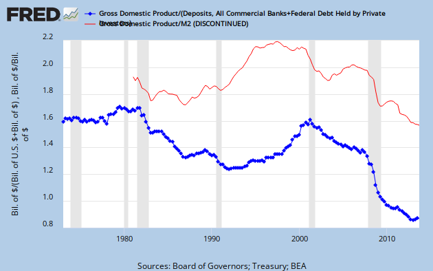 |
| Figure. 5. Money Supply Velocity found from GpMS and M2. |
The Government Provided Money Supply graphs compared to M2 graphs show many differences. These differences can be expected to be the subject of future post on this blog.
Monday, September 9, 2013
Federal Debt and Bank Expansion of the Money Supply
It is widely accepted that Fractional Reserve Banking allows bank loans based on deposits. Considering banks as a whole, any loan creates a new deposit without reducing the deposit of any other customer. The lending bank creates a new asset (a contract to repay) and assumes a new liability (an obligation to restore full value of money to all depositors) in exchange for making this loan and deposit available.
Once expanded by a loan, an increase in available deposits remains in the system as an expanded money supply until the loan is repaid.
If there were no limits to this process, the increased value of all deposits could be used as justification for increased loans. A new loan would equal a new deposit automatically so would there be no need for deposits to precede loans. Loans and deposits could be created simultaneously. This is prevented with limits.
In the United States, the Federal Reserve legally requires banks to hold reserves, currently 10% of all demand deposits. This effectively limits loans to 90% of deposits and creates a limit to deposit expansion. A 10% reserve allows a theoretical expansion of ten times the original deposit.
If the discussion stopped here, we would expect bank loans to be about 10 times reported deposits but data available from the Federal Reserves indicates that the ratio is dramatically less than an average of 1:1. What is going on?
The logic of money supply expansion has one important precondition: The borrowed money must be available to be loaned again. This precondition is fulfilled theoretically by assuming that the loan-based-deposit is spent into the system and then continues to exist someplace as an account entry until the loan is repaid. The single bank equivalent is a loan which once spent, comes back to the bank in a closed system, such as a bank on an isolated island. In both cases, the loan-based-deposit could be used as a base a second, then third time, and so on. The precondition is considered completed.
This precondition may not be met in the United States Economy. Follow the path of a loan-based-deposit as it is spent. Until it gets into the hands of savers, it moves very quickly through the hands of the private economy and government, moving from bank to bank.. Fast moving money is extremely risky for use as a monetary base. A bank would certainly not want to lend money based on a deposit that might only reside in the bank for one day! The large number of banks in the United States acts like a divider of the whole-bank concept, negating the expansion precondition of stable availability. Only the initial expansion is certain, and this is an expansion of two (a doubling), not ten.
As previously mentioned, even a doubling is more expansion than is indicated by Federal Reserved Data. The data suggests that loans are nearly always much less than deposits, barely exceeding a 1:1 ratio just prior to recessions. Does this suggest that the system is operated without limits? No, there is another path that accounts for the less than 1:1 ratio.
The Federal Government has run a deficit for most of the last 50 years. Most of the deficit is funded with money borrowed from the private economy. Government borrows (first) the excess expansion from bank loans and then, if more is needed, from itself acting through the Federal Reserve. Finally, Government purchases from the private economy, thereby providing money for future loans.
The result can be tracked using Federal Reserve Data. About half the expanded money supply is held in banks as deposits. The second half is held in the form of Federal Debt (Note 1.) which is near money and accepted at face value for purposes of complying with Reserve Requirements. Figure 2 shows the sum of bank deposits added to Federal Debt, which will be about double loans at banks, on the long term average.
Once expanded by a loan, an increase in available deposits remains in the system as an expanded money supply until the loan is repaid.
If there were no limits to this process, the increased value of all deposits could be used as justification for increased loans. A new loan would equal a new deposit automatically so would there be no need for deposits to precede loans. Loans and deposits could be created simultaneously. This is prevented with limits.
In the United States, the Federal Reserve legally requires banks to hold reserves, currently 10% of all demand deposits. This effectively limits loans to 90% of deposits and creates a limit to deposit expansion. A 10% reserve allows a theoretical expansion of ten times the original deposit.
If the discussion stopped here, we would expect bank loans to be about 10 times reported deposits but data available from the Federal Reserves indicates that the ratio is dramatically less than an average of 1:1. What is going on?
 |
| Figure 1. Ratio of bank loans to deposits is unexpectedly less than 1:1 on an average. |
This precondition may not be met in the United States Economy. Follow the path of a loan-based-deposit as it is spent. Until it gets into the hands of savers, it moves very quickly through the hands of the private economy and government, moving from bank to bank.. Fast moving money is extremely risky for use as a monetary base. A bank would certainly not want to lend money based on a deposit that might only reside in the bank for one day! The large number of banks in the United States acts like a divider of the whole-bank concept, negating the expansion precondition of stable availability. Only the initial expansion is certain, and this is an expansion of two (a doubling), not ten.
The Federal Government has run a deficit for most of the last 50 years. Most of the deficit is funded with money borrowed from the private economy. Government borrows (first) the excess expansion from bank loans and then, if more is needed, from itself acting through the Federal Reserve. Finally, Government purchases from the private economy, thereby providing money for future loans.
The result can be tracked using Federal Reserve Data. About half the expanded money supply is held in banks as deposits. The second half is held in the form of Federal Debt (Note 1.) which is near money and accepted at face value for purposes of complying with Reserve Requirements. Figure 2 shows the sum of bank deposits added to Federal Debt, which will be about double loans at banks, on the long term average.
 |
Figure 2. When Federal Debt held by the public is added to bank deposits, the relationship to bank loans is about 2:1 on the average. This relationship builds the case for considering Federal Debt as part of money supply.
|
This post will conclude by pointing out that bank loans result in deposits. Each bank loan has an original deposit that preceded the loan so we could expect to locate two deposits for each loan. Surprisingly, the expected result of two deposits to one loan is not observable in Federal Reserve Data. The deposits not-accounted-for have been loaned to the Federal Government and can be found accounted as Federal Debt.
Being debt of government and very safe assets, these missing deposits in the form of Federal Debt can legally be counted as bank reserves. These missing deposits in the form of Federal Debt could also be counted as part of the national money supply.
Note 1. The label "Federal Debt" is used generically but a more precise definition would be "Federal Debt held by the public". Federal Debt as a trust fund obligation is not counted. Federal Debt held by the public, as defined in this post, is accounted by the Federal Reserve as data series FDHBPIN.
Sunday, September 1, 2013
The Widow's Cruse and Derivative Loans
Many bloggers are currently writing about the widow's cruse and the relationship of bank loans to money supply. My latest tack is to consider the changes that would occur if an economy moved from a limited-bank economy to an economy with banks as we know them.
In this model, the initial economy has a completely fiat currency with no derivative loans allowed. Here I define derivative loans as "loans from an institution that result in at least two parties having claim on the same underlying asset".
The initial economy can have banks but all loans are single party loans. That is, all loans are clearly tied between lender and borrower, with lender well aware that borrower is spending the lenders money. Any expansion of the money supply under this system must come from the sponsor of the fiat money supply.
The total amount of money in circulation can be measured by the difference between total amount issued less the amount borrowed back by the sponsor as the sponsor strives to maintain value of a fiat currency. This difference should be slightly less than the amount on deposit at institutions because some portion would be held in wallets and under mattresses.
Now we will change the model to allow derivative loans (DL) by banks. In this modified model, loans can be based on the deposits in the bank. Money sitting in bank storage, similar to sitting under a mattress, can be put to use and can stimulate an economy.
DL loans have three very important properties:
(1) When the loaned money is spent, it will result in increased deposits owned by third parties. The third parties are unlikely to deposit at the bank making the DL loan, but are likely to deposit at banks acting within the fiat money system. The result can be measured initially from an increase in bank deposits by the amount of the loan (again excepting part held in wallets and under mattresses).
(2) It is impossible to distinguish between Original Currency (OC) and DL. This creates a situation of increasing DL based deposits. This process has no upper limit. Ever more owners can claim ever increasing deposits in accounts.
(3) Transfers between banks are limited to transfers of OC. This is an extremely important limitation. Assume that a deposit holder writes a check and the check is deposited to another bank. The second bank does not automatically credit to the bearer's deposit account. Instead, the second bank issues a draw against the currency assets of the bank of check origin. Two conditions must then be satisfied:
(3a) The check deposit owner must have funds adequate to cover the check.
(3b) The bank must have currency adequate to cover the check. This currency must be currency originally issued by government (OC), not a DL deposit.
The effect of properties 2 and 3b create a banking dilemma: Ever more depositors have ever increasing claims on a fixed amount of OC! Unchecked, this dilemma will end with collapse of the banking system when it becomes obvious that the system can not satisfy the the claims of all depositors with OC.
Returning to the blog question of widow's cruse, it would seem that property 2 grants that generosity, the banks have a widows's cruse. Unfortunately, property 3b would indicate that no cruse at all could ever exist between banks.
If these properties are correct, then important effects on money supply measurement necessarily follow:
A. Original Currency issued by the government is the only money supply available. This can be measured as the difference between government expenses and government receipts. Continuous deficits act to continuously increase the money supply.
B. Original Currency exists like a "hot potato". It does not disappear from public use unless removed by government, principally by running a budget surplus as when taxes exceed expenses. Government borrowing does not extinguish the OC, it merely puts it back into motion. Measurement of OC by adding the deposits of all banks should closely match the amount of government debt held by the public. Differences between deposits and debt held by the public should be principally due to central bank efforts to control currency value.
C. The sum of all outstanding loans has no bearing on money supply measurement. On the other hand, the sum of all outstanding loans is a vital measurement of the need by the public for future currency for loan payments. Currency tied up in the hands of deposit holders is no guaranty that currency will be available to borrowers for loan payments.
D. The change in bank loans is a measurement of money put into motion where it can be expected to increase GDP. If government is repeatedly running a deficit, an increase in loans may increase tax income, thus lowering the needed level of borrowing to meet a preset budget. This effect resulted in a rare government budget surplus in the late 1990's. This same effect created a need for massive government borrowing beginning in about 2007 when loan failures forced massive government borrowing to maintain then existing government spending.
My conclusion is that the widow's cruse does exist like a rainbow does exist. Unfortunately, the widow's cruse only continues while conditions are correct, then it vanishes.
Thursday, August 1, 2013
Modeling the Delayed Effects of Investment
In this post, I will suggest a model of the delayed effects of investment. A convenient point of entry is the excellent post by Nick Edmonds found at http://monetaryreflections.blogspot.co.uk/2013/07/bank-lending-and-non-bank-lending-model.html .
Edmonds correctly arrives at the equation
|
ΔL + ΔB + α0 |
||
|
1. Y |
= |
------------------ |
|
Eq |
( 1 - α1 ) |
where Y is income, ∆L + ∆B is the change in bank lending plus the change in lending by bonds, aₒ is base consumer spending and a₁ is an adjustment factor relating all the terms. This simple equation has the effect of hiding the long term effects of bank and bond investing.
We can separate and examine the long and short term effects of bank lending plus lending by bonds by defining lending as money that is borrowed and would result in spending that would count toward national income as measured by GDP. This is a severe limitation that we enforce by placing a negative limit on equation 1. To add this limit to equation 1, we would rewrite it to read
|
ΔL + ΔB + α0 |
||
|
2. Y |
= |
------------------- Limit ∆L + ∆B > zero. |
|
Eq |
( 1 - α1 ) |
In other words, bank and bond lending cannot be negative or below zero. If they were negative, they would represent a transaction that is not counted as income but, instead, would be an investment transaction which is not counted as part of GDP.
We will avoid the need for limits by defining our terms carefully. Here, we depart from the definitions of Edmonds, except for the Y term which is commonly used to identify income.
We will narrowly define investment loans from bonds and bank loans as being new loans and bonds, as contrasted to refunding or roll-over loans or bonds. New loans and bonds are anticipated to be spent on new plant, labor, material or other item that would be counted as adding to the national GDP calculation. We label new bank loans NBL and new bond issues NBI.
We will assume that every income reporting period is expected to have a different consumer spending base. We label the annual consumer spending base as ACSB.
Up to this point, we have identified two sources of consumer income, borrowing (NBL + NBI) and base spending (ACSB). We will follow Edmonds by ignoring the effects of Government until a later posting. If we also ignore the delayed effects of new loan spending, we can write
3. Y = NBL + NBI + ACSB.
From equation 3, we can see that national consumer income is at least new investment spending plus base consumer spending.
Now we will examine the delayed effects of new money. New investment spending moves money from the hands of savers into the hands of workers and materials providers. This movement into new hands is likely to result in additional spending at some unforeseeable time in the future. New hands holding new money will change the base consumer spending pattern Y both in the current time period and future time periods. To model this change in the most recent time period, equation 3 will be supplemented with the term a₂ times the value of new loans and new bonds (a₂ * ( NBL +NBI), where a₂ is the expansion factor for new money . We will write
4. Y = a₂*(NBL + NBI) + NBL + NBI + ACSB .
From equation 4, we can see that national consumer income is at least the factor a₂ times new investment spending, plus new investment spending, plus base consumer spending.
Investment in the next income period may not contain any new investment income but it is highly likely that investment income from the previous period will carry over into subsequent periods. If equation 4 is used to predict an income for a future Y₁ with no future investment, we could write
5. Y₁ = a₃*(NBL + NBI) + ACSB
where a₃ is the revised constant for the no-investment period. NBL, NBI, and ACSB are equal to identical terms from the previous year’s calculation.
More can be done with this model as represented by equation 4. Government can be added to show the effect of changing the base money supply. ACSB can be traced back in time in an attempt to establish a base consumer spending level or find the annual value of a₂. It is expected that these and additional subjects will be covered in future postings.
Subscribe to:
Posts (Atom)